class: center, middle, inverse, title-slide # Laboratorio Bio-demografico ## Lezione 4 ### Nicola Barban <br> Alma Mater Studiorum Università di Bologna <br> Dipartimento di Scienze Statistiche ### 23 Febbraio 2021<br> <img src="../img/UniBo-Universita-di-Bologna.png" style="width:20.0%" /> --- # Outline - Tidyverse - Trasformazione Dati - Reshape - Merge - %>% Pipes - Incidenza e Prevalenza. Letalità e Mortalità. - Dati Covid. Italia e altri paesi. --- # Tidyverse {width=80%} --- # cos'è tidyverse? Collezione di R packages per modellare, trasformare e visualizzare dati * ggplot2, * dplyr, * tidyr, * readr, * purrr, * tibble, * stringr, and * forcats https://www.tidyverse.org --- # Tidy Dataset Definizione: 1. Each variable must have its own column 2. Each observation must have its own row 3. Each value must have its own cell --- # Esempio .pull-left[ ```r library(tidyverse) table1 ``` ``` ## # A tibble: 6 x 5 ## country year cases population rate ## <chr> <int> <int> <int> <dbl> ## 1 Afghanistan 1999 745 19987071 0.0373 ## 2 Afghanistan 2000 2666 20595360 0.129 ## 3 Brazil 1999 37737 172006362 0.219 ## 4 Brazil 2000 80488 174504898 0.461 ## 5 China 1999 212258 1272915272 0.167 ## 6 China 2000 213766 1280428583 0.167 ``` ] .pull-right[  ] --- # Not a tidy dataset ```r table2 ``` ``` ## # A tibble: 12 x 4 ## country year type count ## <chr> <int> <chr> <int> ## 1 Afghanistan 1999 cases 745 ## 2 Afghanistan 1999 population 19987071 ## 3 Afghanistan 2000 cases 2666 ## 4 Afghanistan 2000 population 20595360 ## 5 Brazil 1999 cases 37737 ## 6 Brazil 1999 population 172006362 ## 7 Brazil 2000 cases 80488 ## 8 Brazil 2000 population 174504898 ## 9 China 1999 cases 212258 ## 10 China 1999 population 1272915272 ## 11 China 2000 cases 213766 ## 12 China 2000 population 1280428583 ``` --- # library(dplyr) Package per trasformare dati [cheatsheet](https://github.com/rstudio/cheatsheets/blob/master/data-transformation.pdf) --- # Creare nuove variabili ```r table1$rate<-1000*table1$cases/table1$population table1 ``` ``` ## # A tibble: 6 x 5 ## country year cases population rate ## <chr> <int> <int> <int> <dbl> ## 1 Afghanistan 1999 745 19987071 0.0373 ## 2 Afghanistan 2000 2666 20595360 0.129 ## 3 Brazil 1999 37737 172006362 0.219 ## 4 Brazil 2000 80488 174504898 0.461 ## 5 China 1999 212258 1272915272 0.167 ## 6 China 2000 213766 1280428583 0.167 ``` --- # Creare nuove variabili (tidyverse) ```r table1 <- mutate(table1, rate= 1000*cases/population) table1 ``` ``` ## # A tibble: 6 x 5 ## country year cases population rate ## <chr> <int> <int> <int> <dbl> ## 1 Afghanistan 1999 745 19987071 0.0373 ## 2 Afghanistan 2000 2666 20595360 0.129 ## 3 Brazil 1999 37737 172006362 0.219 ## 4 Brazil 2000 80488 174504898 0.461 ## 5 China 1999 212258 1272915272 0.167 ## 6 China 2000 213766 1280428583 0.167 ``` --- # operatore **%>%** Operatore pipe %>% * ambiente macOS: `CMD+Shift+M` * ambiente Windows: `CTRL+Shift+M` * Funziona esattamente come una tubatura: + elemento (input) in ingresso viene dirottato verso l'istruzione/output --- # Creare nuove variabili ### tidyverse usando pipes ```r table1 <- table1 %>% * mutate(rate= 1000*cases/population) table1 ``` ``` ## # A tibble: 6 x 5 ## country year cases population rate ## <chr> <int> <int> <int> <dbl> ## 1 Afghanistan 1999 745 19987071 0.0373 ## 2 Afghanistan 2000 2666 20595360 0.129 ## 3 Brazil 1999 37737 172006362 0.219 ## 4 Brazil 2000 80488 174504898 0.461 ## 5 China 1999 212258 1272915272 0.167 ## 6 China 2000 213766 1280428583 0.167 ``` --- ```r # compute cased per year table1 %>% count(year, wt = cases) ``` ``` ## # A tibble: 2 x 2 ## year n ## * <int> <int> ## 1 1999 250740 ## 2 2000 296920 ``` --- ```r # pipe and ggplot table1 %>% ggplot( aes(x=year, y=cases, color=country)) + geom_line()+ geom_point() ``` <img src="lezione4_files/figure-html/unnamed-chunk-7-1.png" width="40%" /> --- # Filter seleziona **osservazioni** ```r library(gapminder) gapminder_asia <- gapminder %>% filter(continent=="Asia", year>1985) #View(gapminder_asia) ``` --- ```r gapminder_asia ``` ``` ## # A tibble: 165 x 6 ## country continent year lifeExp pop gdpPercap ## <fct> <fct> <int> <dbl> <int> <dbl> ## 1 Afghanistan Asia 1987 40.8 13867957 852. ## 2 Afghanistan Asia 1992 41.7 16317921 649. ## 3 Afghanistan Asia 1997 41.8 22227415 635. ## 4 Afghanistan Asia 2002 42.1 25268405 727. ## 5 Afghanistan Asia 2007 43.8 31889923 975. ## 6 Bahrain Asia 1987 70.8 454612 18524. ## 7 Bahrain Asia 1992 72.6 529491 19036. ## 8 Bahrain Asia 1997 73.9 598561 20292. ## 9 Bahrain Asia 2002 74.8 656397 23404. ## 10 Bahrain Asia 2007 75.6 708573 29796. ## # … with 155 more rows ``` --- # Select seleziona **variabili** ```r library(gapminder) gapminder_LE <- gapminder %>% select(country, continent, year, lifeExp) #View(gapminder_LE) gapminder_LE ``` ``` ## # A tibble: 1,704 x 4 ## country continent year lifeExp ## <fct> <fct> <int> <dbl> ## 1 Afghanistan Asia 1952 28.8 ## 2 Afghanistan Asia 1957 30.3 ## 3 Afghanistan Asia 1962 32.0 ## 4 Afghanistan Asia 1967 34.0 ## 5 Afghanistan Asia 1972 36.1 ## 6 Afghanistan Asia 1977 38.4 ## 7 Afghanistan Asia 1982 39.9 ## 8 Afghanistan Asia 1987 40.8 ## 9 Afghanistan Asia 1992 41.7 ## 10 Afghanistan Asia 1997 41.8 ## # … with 1,694 more rows ``` --- # combinare diverse operazioni ```r library(gapminder) gapminder_selezione <- gapminder %>% select(country, continent, year, lifeExp) %>% filter(continent=="Asia", year>1985) str(gapminder_selezione) ``` ``` ## tibble [165 × 4] (S3: tbl_df/tbl/data.frame) ## $ country : Factor w/ 142 levels "Afghanistan",..: 1 1 1 1 1 8 8 8 8 8 ... ## $ continent: Factor w/ 5 levels "Africa","Americas",..: 3 3 3 3 3 3 3 3 3 3 ... ## $ year : int [1:165] 1987 1992 1997 2002 2007 1987 1992 1997 2002 2007 ... ## $ lifeExp : num [1:165] 40.8 41.7 41.8 42.1 43.8 ... ``` ```r #View(gapminder_selezione) ``` --- # Arrange Ordina le osservazioni del dataset ```r table1 %>% arrange( desc( population)) ``` ``` ## # A tibble: 6 x 5 ## country year cases population rate ## <chr> <int> <int> <int> <dbl> ## 1 China 2000 213766 1280428583 0.167 ## 2 China 1999 212258 1272915272 0.167 ## 3 Brazil 2000 80488 174504898 0.461 ## 4 Brazil 1999 37737 172006362 0.219 ## 5 Afghanistan 2000 2666 20595360 0.129 ## 6 Afghanistan 1999 745 19987071 0.0373 ``` --- # wide and long data format 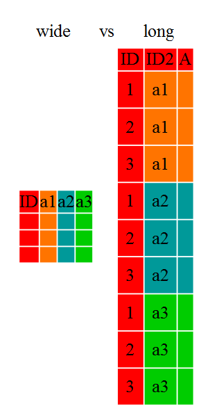 --- # pivot_longer() or gather() From **wide** to **long** 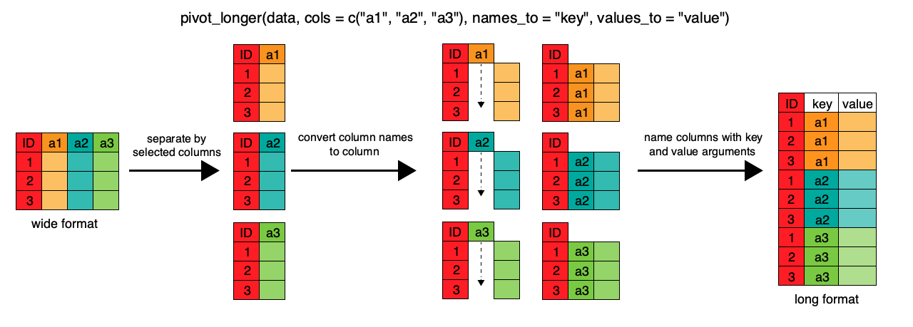 --- ```r vignette("pivot") ``` --- ```r relig_income ``` ``` ## # A tibble: 18 x 11 ## religion `<$10k` `$10-20k` `$20-30k` `$30-40k` `$40-50k` `$50-75k` `$75-100k` `$100-150k` ## <chr> <dbl> <dbl> <dbl> <dbl> <dbl> <dbl> <dbl> <dbl> ## 1 Agnostic 27 34 60 81 76 137 122 109 ## 2 Atheist 12 27 37 52 35 70 73 59 ## 3 Buddhist 27 21 30 34 33 58 62 39 ## 4 Catholic 418 617 732 670 638 1116 949 792 ## 5 Don’t k… 15 14 15 11 10 35 21 17 ## 6 Evangel… 575 869 1064 982 881 1486 949 723 ## 7 Hindu 1 9 7 9 11 34 47 48 ## 8 Histori… 228 244 236 238 197 223 131 81 ## 9 Jehovah… 20 27 24 24 21 30 15 11 ## 10 Jewish 19 19 25 25 30 95 69 87 ## 11 Mainlin… 289 495 619 655 651 1107 939 753 ## 12 Mormon 29 40 48 51 56 112 85 49 ## 13 Muslim 6 7 9 10 9 23 16 8 ## 14 Orthodox 13 17 23 32 32 47 38 42 ## 15 Other C… 9 7 11 13 13 14 18 14 ## 16 Other F… 20 33 40 46 49 63 46 40 ## 17 Other W… 5 2 3 4 2 7 3 4 ## 18 Unaffil… 217 299 374 365 341 528 407 321 ## # … with 2 more variables: `>150k` <dbl>, `Don't know/refused` <dbl> ``` --- ```r relig_income %>% pivot_longer(cols=!religion, names_to = "income", values_to = "count") ``` ``` ## # A tibble: 180 x 3 ## religion income count ## <chr> <chr> <dbl> ## 1 Agnostic <$10k 27 ## 2 Agnostic $10-20k 34 ## 3 Agnostic $20-30k 60 ## 4 Agnostic $30-40k 81 ## 5 Agnostic $40-50k 76 ## 6 Agnostic $50-75k 137 ## 7 Agnostic $75-100k 122 ## 8 Agnostic $100-150k 109 ## 9 Agnostic >150k 84 ## 10 Agnostic Don't know/refused 96 ## # … with 170 more rows ``` --- # pivot_longer() * il primo argomento `data` è il dataset su cui fare reshape: `relig_income`. *In questo caso viene passsato da %>% * * il secondo argomento descrive le colonne che devono essere trasformate. In questo caso: *tutte tranne `religion` * * Il terzo argomento `names_to` da il nome alla nuova variabile creata partendo dal nome delle variabili presenti nel dataset *wide* * Il quarto argomento `values_to` da il nome alla variabile creata partendo dai valori nel dataset *wide* --- # pivot_wider() or spread() From **long** to **wide** 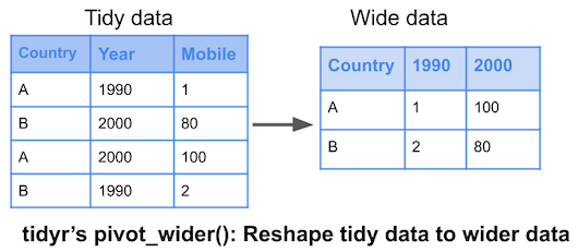 --- ```r gapminder_selezione ``` ``` ## # A tibble: 165 x 4 ## country continent year lifeExp ## <fct> <fct> <int> <dbl> ## 1 Afghanistan Asia 1987 40.8 ## 2 Afghanistan Asia 1992 41.7 ## 3 Afghanistan Asia 1997 41.8 ## 4 Afghanistan Asia 2002 42.1 ## 5 Afghanistan Asia 2007 43.8 ## 6 Bahrain Asia 1987 70.8 ## 7 Bahrain Asia 1992 72.6 ## 8 Bahrain Asia 1997 73.9 ## 9 Bahrain Asia 2002 74.8 ## 10 Bahrain Asia 2007 75.6 ## # … with 155 more rows ``` --- ```r gapminder_selezione %>% pivot_wider(id=country, names_from=year, values_from=lifeExp) ``` ``` ## # A tibble: 33 x 6 ## country `1987` `1992` `1997` `2002` `2007` ## <fct> <dbl> <dbl> <dbl> <dbl> <dbl> ## 1 Afghanistan 40.8 41.7 41.8 42.1 43.8 ## 2 Bahrain 70.8 72.6 73.9 74.8 75.6 ## 3 Bangladesh 52.8 56.0 59.4 62.0 64.1 ## 4 Cambodia 53.9 55.8 56.5 56.8 59.7 ## 5 China 67.3 68.7 70.4 72.0 73.0 ## 6 Hong Kong, China 76.2 77.6 80 81.5 82.2 ## 7 India 58.6 60.2 61.8 62.9 64.7 ## 8 Indonesia 60.1 62.7 66.0 68.6 70.6 ## 9 Iran 63.0 65.7 68.0 69.5 71.0 ## 10 Iraq 65.0 59.5 58.8 57.0 59.5 ## # … with 23 more rows ``` --- # From long to wide and from wide to long ```r gapminder_selezione %>% pivot_wider(id=country, names_from=year, values_from=lifeExp) %>% pivot_longer(cols=!country, names_to = "year", values_to = "lifeExp") ``` ``` ## # A tibble: 165 x 3 ## country year lifeExp ## <fct> <chr> <dbl> ## 1 Afghanistan 1987 40.8 ## 2 Afghanistan 1992 41.7 ## 3 Afghanistan 1997 41.8 ## 4 Afghanistan 2002 42.1 ## 5 Afghanistan 2007 43.8 ## 6 Bahrain 1987 70.8 ## 7 Bahrain 1992 72.6 ## 8 Bahrain 1997 73.9 ## 9 Bahrain 2002 74.8 ## 10 Bahrain 2007 75.6 ## # … with 155 more rows ``` --- # Ggplot preferisce il formato *long* * Posso usare varie categorie per definire *aestehics* in ggplot * Ad esempio: ```r ggplot(iris, aes(x=Sepal.Length, y=Sepal.Width, color=Species)) + geom_point(size=6) + theme_dark() ``` <img src="lezione4_files/figure-html/unnamed-chunk-19-1.png" width="40%" /> --- # Summarise Data Derivare statistiche aggregate da un dataset  --- # Summarise Data **per gruppi** Derivare statistiche aggregate da un dataset  --- # Esempio ```r iris %>% group_by(Species) %>% summarise(Lunghezza.Media=mean(Sepal.Length), N=length(Sepal.Length)) ``` ``` ## # A tibble: 3 x 3 ## Species Lunghezza.Media N ## * <fct> <dbl> <int> ## 1 setosa 5.01 50 ## 2 versicolor 5.94 50 ## 3 virginica 6.59 50 ``` --- # Combine datasets **Full Join** Unire diversi datasets. *Unione datasets*  --- # Combine datasets **Inner Join** Unire diversi datasets. *Intersezione datasets*  --- # Combine datasets **Left Join** Unire diversi datasets.  --- # Combine datasets **Right Join** Unire diversi datasets.  --- # Riassunto  --- # Le misure di frequenza delle malattie ### Prevalenza * **l'insieme di tutti i casi esistenti** di una specifica patologia in un determinato momento e in una determinata popolazione. - *il numero dei nuovi attuali positivi misura la **variazione di prevalenza della positività**, che si traduce in una variazione del carico sul sistema sanitario.* -- * **la comparsa di nuovi casi** di una specifica patologia in una popolazione in un determinato periodo di tempo - *Velocità con cui la malattia si diffonde* --- # Prevalenza e incidenza | PREVALENZA | INCIDENZA | |---------------------------------------------------------------------|------------------------------------------------------------------------------| | probabilità di avere una malattia | probabilità di sviluppare una malattia | | il numeratore comprende tutti i malati | il numeratore comprende solo i nuovi casi in un determinato periodo di tempo | | il denominatore comprende gli individui ammalati e quelli a rischio | il denominatore comprende gli individui a rischio e inizialmente sani | | in un dato istante, rilevabile con una sola indagine | richiede almeno due indagini distanziate nel tempo | | utile per valutare l’impatto di una malattia in una popolazione | utile per valutare l’estendersi di una malattia | --- # Letalità e Mortalità * Il **tasso di letalità** è il rapporto tra il numero delle persone decedute a causa della malattia e il totale dei malati. --> *Case Fatality Rate CFR* * Il **tasso di mortalità** calcola quante persone sono morte sul totale delle persone esposte, cioè sugli abitanti del nostro paes .-- > * Mortality Rate* --- # Ourl World In Data https://ourworldindata.org/coronavirus-data-explorer?time=earliest..latest&country=OWID_WRL~USA~ITA~BRA~ESP~SWE~DEU~IND~IRN~KOR~NZL&region=World&cfrMetric=true&interval=total&aligned=true&hideControls=true&smoothing=0&pickerMetric=location&pickerSort=asc <iframe src="https://ourworldindata.org/coronavirus-data-explorer?time=earliest..latest&country=OWID_WRL~USA~ITA~BRA~ESP~SWE~DEU~IND~IRN~KOR~NZL&region=World&cfrMetric=true&interval=total&aligned=true&hideControls=true&smoothing=0&pickerMetric=location&pickerSort=asc" loading="lazy" style="width: 100%; height: 600px; border: 0px none;"></iframe> --- # Portale COVID https://www.covid19dataportal.it/data_types/health_data/data/ --- # Dati protezione civile https://github.com/pcm-dpc/COVID-19  --- # Dati andamento covid https://github.com/pcm-dpc/COVID-19/blob/master/dati-andamento-covid19-italia.md  # Dati internazionali https://ourworldindata.org/coronavirus-data-explorer?yScale=log&zoomToSelection=true&minPopulationFilter=1000000&country=USA~GBR~BRA~IND~DEU~MEX~CHL~ZAF~COL~KOR~NOR~URY~ITA&region=World&deathsMetric=true&interval=smoothed&aligned=true&smoothing=7&pickerMetric=location&pickerSort=asc <iframe src="https://ourworldindata.org/coronavirus-data-explorer?yScale=log&zoomToSelection=true&minPopulationFilter=1000000&country=USA~GBR~BRA~IND~DEU~MEX~CHL~ZAF~COL~KOR~NOR~URY~ITA&region=World&deathsMetric=true&interval=smoothed&aligned=true&smoothing=7&pickerMetric=location&pickerSort=asc" loading="lazy" style="width: 100%; height: 600px; border: 0px none;"></iframe> -- # DATI AGGIORNATI DA *OUR WORLD IN DATA* https://github.com/owid/covid-19-data/tree/master/public/data  --- # EUROPEAN DATA https://www.ecdc.europa.eu/en/geographical-distribution-2019-ncov-cases  --- # Dati vaccinazioni https://github.com/italia/covid19-opendata-vaccini